The major factors that determine the labour forecast are the volume forecast, labour standards, and labour forecast limits.
The labour forecast indicates how much labour is required to meet the amount of business predicted in the volume forecast. The labour forecast calculates total labour hours per day per job for a week. The labour forecast converts the labour hours into the number of employees, by job, who are needed to meet the demand in each 15-minute interval per day.
Note: The Forecast Planner automatically adjusts the forecast for labour that crosses the week divide.
From the labour forecast, the Schedule Generator Creates or assigns shifts based on the workload, shift templates or profiles, employee and organizational rules, and engine settings. analyses individual employees and schedule rules Defines restrictions and requirements to ensure that a schedule meets certain criteria. and creates a schedule, one week at a time, for each job in a selected location.
In addition to the data from the volume drivers, the labour forecast requires three kinds of drivers that do not depend on volume:
- Static drivers – Based on physical values that do not vary with business volume, such as the size of the shop. For example, the larger the shop, the more security and maintenance staff are required.
- Custom drivers – Include labour data that does not vary by volume or by any static value; for example, the amount of training that new employees require.
- Fixed frequency drivers – Specify the number of times an activity occurs in a specific time period; for example, printing a report once a day takes 5 minutes.
Note: Fixed frequency drivers are defined when you configure labour standards.
To get the most accurate labour forecast at the job level, the Forecast Planner requires the smallest possible measurable unit of work for its calculations; for example, 4 seconds to scan an item at the register.
Labour standards contain the time values for the amount of labour required to complete specific tasks, such as scanning an item. The Forecast Planner multiplies the time value in each labour standard by the appropriate driver data to calculate the labour requirement to complete specific tasks. The system can then determine how many hours of labour are required for the jobs that need to be scheduled.
Some labour standards are driven by volumes. For example, it takes a certain amount of time to scan so many items at a register. The labour needed to scan all the items at a register is driven by this amount of time multiplied by the number of items that are expected to be going through the register during the time period of the labour forecast.
Other labour standards are driven by criteria that are not based on volumes. Some examples of these include:
- A “floor sweep” standard that defines the amount of time to sweep the amount of floor space in your shop.
- A “train new employee” standard that defines how long it takes to train a newly hired employee. This type of labour standard requires a custom driver, which defines how many new employees need to be trained in the upcoming week.
- A “run report” standard that defines how long it takes to run a report that is run once per day every day.
Labour standards are associated with tasks.
Labour standards are grouped into tasks. For example, the labour standards for callback, handle complaint, exterior event, and so on, can be grouped into the task of customer service.
One or more tasks is assigned to a task group. Each job included in the labour forecast is associated with a task or task group. Only jobs that have a labour standard associated with them are included in the labour forecast.
The Combined Distribution feature lets you combine labour standards for a task so that the labour is distributed more evenly.
Combined Distribution allows you to combine labour standards for a task in order to achieve more even labour distribution. This option ensures that any fractional head counts that occur during the labour calculation process for individual labour standards are accumulated, and then redistributed to the specified job within the configured labour period.
The combined distribution functionality
- Generates a more evenly distributed labour forecast curve for a day
- Minimises gains and losses in labour forecast hours due to rounding
- Uses planned resources – both demand driven and fixed – more effectively to honour minimum requirements defined in labour forecast limits
The combined labour distribution option works well when
- Labour standards use Apply Rounding
- The combined labour standards are configured to Distribute by Traffic Pattern.
The combined distribution option does not work for
- Labour standards that are configured to Distribute Evenly with the option Spread Remainder Left or Spread Remainder right selected.
- Time Independent Labour Standards
In the event that one or more labour standards selected for combined distribution have Spread Remainder Left or Spread Remainder Right selected, the system automatically overrides the labour standard configuration to Apply Rounding. If this is done, this is noted in the log file.
Any fractional head count that is generated during the labour calculation process is added, by job, to a daily resource pool. Rather than rounding, for example, 3.5 of a head count requirement up to 4 or down to 3, the system puts the 0.5 into the resource pool. This labour is then distributed within the combined distribution time period for the labour in the following priority order:
- Ensure minimum requirements are met.
- Ensure that any fractional head count in any 15-minute interval is rounded.
- Make sure that any resources that were lost during the labour calculation process for an individual labour standard is accumulated. Distribute any remaining resources using the selected distribution method:
- Spread right – Spreads remaining resources in the resource pool starting at the end of the distribution time period, working toward the beginning of the distribution period until resources are used up.
- Spread left – Spreads the remaining resources in the resource pool starting at the beginning of the distribution time period, working toward the end of the distribution period until resources are used up.
- Optimal spread – Redistributes any remaining labour to the appropriate time periods in the labour forecast curve. This ensures that the final labour forecast curve for the job is smoothed.
A simple example of the combined labour distribution concept is shown using five fixed labour standards for a shop clerk. Assuming that each of these labour standards has the same labour period of one hour (9 A.M. – 10 A.M.) on a given day, the raw labour forecast generated for each interval of the day is as follows:
|
Labour Standard |
9:00 A.M. |
9:15 A.M. |
9:30 A.M. |
9:45 A.M. |
|
1 |
1.5 |
1.5 |
1.5 |
1.5 |
|
2 |
2.0 |
2.0 |
2.0 |
2.0 |
|
3 |
2.5 |
2.5 |
2.5 |
2.5 |
|
4 |
1.5 |
1.5 |
1.5 |
1.5 |
|
5 |
1.75 |
1.75 |
1.75 |
1.75 |
|
Total (raw head count) |
9.25 |
9.25 |
9.25 |
9.25 |
If we do not apply combined labour distribution, then the raw head count of 9.25 for the day is rounded down to 9 in the final labour forecast. Hence, the overall loss in the labour forecast for the day is 0.25 hours, or 15 minutes.
If we do apply combined labour distribution to the five labour standards in the example, then each 15-minute interval contributes 2.25 head count to the daily resource pool. Hence, the size of the resource pool for the day is 2.25 x 4 = 9 head count.
If the Spread remainder left combined distribution method is used, then labour distribution from the resource pool is:
|
Pass |
9:00 A.M. |
9:15 A.M. |
9:30 A.M. |
9:45 A.M. |
Pool size |
|
Before CLD |
7 |
7 |
7 |
7 |
9 |
|
First pass |
8 |
8 |
8 |
8 |
5 |
|
Second pass |
9 |
9 |
9 |
9 |
1 |
|
Third pass |
10 |
9 |
9 |
9 |
0 |
the final labour forecast is:
|
9:00 A.M. |
9:15 A.M. |
9:30 A.M. |
9:45 A.M. |
|
10 |
9 |
9 |
9 |
In this example the final labour forecast after combined distribution is 9.25 hours and we do not get any loss in the labour forecast from rounding.
Labour forecast limits include minimum and maximum labour coverage requirements for jobs and job rounding factors.
- You can set minimum and maximum labour coverage requirements for a job regardless of the amount of business volume that the Forecast Planner calculates. For example you may always want a minimum number of cashiers scheduled no matter how low the volume forecast. And, if you have 13 registers, you probably do not want more than 13 or 14 cashiers scheduled no matter how high the volume forecast.
- You can set a rounding factor for each job. When the labour forecast engine converts forecast hours to head count, a fraction of a person, such as 3.7 people, often results. You can set the point at which to round the head count requirement up, for example, to 4 or down to 3.
The Forecast Planner uses the hours during which a site or department is open for business when it:
- Calculates the traffic pattern
- Creates the labour forecast
Labour standards can be configured to distribute labour requirements relative to a shop’s hours of operation; for example, the labour requirement for setup starts 15 minutes before the shop opens, and clean up runs until 15 minutes after the shop is closed.
Hours of operation can be configured to be regular hours, which are based on standard open and close time for each day of the week. Override hours can be configured to define changes to the standard hours Non-overtime hours that each employee is expected to work. for a specific date, such as a holiday.
Hours of operation are assigned to categories at the department level or above on the business structure. The hours of operation assignments can be effective dated.
All departments in the shop inherit their hours of operation from the site. However, if a department has different hours than a site, it can be assigned to a different set of hours of operation to the department.
Corporate can create an hours of operation and deny a shop the ability to edit it.
Traffic patterns tell the Forecast Planner how to distribute the labour forecast by showing how business volume fluctuates during a day; for example, what times have high volumes, and at what times does volume drop off.
To calculate a traffic pattern, the Forecast Planner uses historical data from volume drivers on similar days in the past. For example, to forecast next Monday, it looks at three points:
- Last Monday – 1630 customers were in the shop between 9 A.M. and 10 A.M.
- Two Mondays ago – 1410 customers were in the shop between 9 A.M. and 10 A.M.
- Three Mondays ago – 1474 customers were in the shop between 9 A.M. and 10 A.M
From this volume driver data, the Forecast Planner can forecast approximately how many customers will be in the store between 9 A.M. and 10 A.M. next Monday.
To distribute the forecasted labour correctly in 15-minute intervals, the Forecast Planner does one of the following:
- Divides the labour requirement evenly across the labour period
- Derives a traffic pattern from actual historical data and the parameters you enter during setup. It then fits the forecasted labour hours under that traffic pattern curve, and divides the curve into 15-minute intervals
-
$ 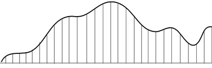
Time in 15-minute intervals
After the labour forecast distributed correctly, the system is ready to find real employees and schedule them to the jobs and shifts that can fulfil the business requirements.
You can export a traffic pattern for shops or departments before you generate the labour forecast. You can compare the 15-minute interval values in the labour forecast to values in your internal reports. If necessary, you can edit the values and then import the values back into the system where they are used when you generate your labour forecast.